M1 DIGIT – Sorbonne Université System Design and
Modeling
Lab I: Running
Simulations and Performance Analysis
The objective of
these practical class works is to become familiar with the analysis of the
performance of a network system via simulations. In these Labs, you will compare the
results obtained by simulations with those obtained by analytical modeling.
IMPORTANT. At the end of each lab (03:50pm), you must send a first version of your lab report. This first version must include all your results of the Lab: Observations, numerical values, and all figures with plots, plus some few texts to answer questions. Afterwards, you will write and send a final report. This final report must complete the texts and include additionally a comprehensive analysis for each result in which you explain carefully your simulation observations in order to provide useful conclusions. The deadline to send this final report is Tuesday, April 01, 2025 before 08:30 am
Poisson/UDP traffic through two links
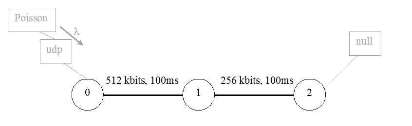
Figure 1: Simple network with two links
Copy the simulation script file lab1.tcl. This tcl script creates the network of Figure 1 for ns2 with the following properties:
· Simulation parameters:
a. It creates the trace file /tmp/out.tr in order to save in the local disk all the events simulated by ns2.
b. Simulation time equals 10000 seconds.
· Traffic parameters:
a. It creates the Poisson traffic generator (see the figure) of parameter λ.
b. The transport protocol is UDP.
c. The size of the packets is 1024 bytes.
· Links parameters:
a. Link 0-1: 512 kbits, propagation delay: 100ms, queue scheduling: FIFO, queue size: 100 packets
b. Link 1-2: 256 kbits, propagation delay: 100ms, queue scheduling: FIFO, queue size: 100 packets
· The random generator takes the initial value from the seed variable given as an input.
(You can take a look at the tcl source code of lab1.tcl but right now do not modify it.)
In order that the ns program can be executed from any terminal, include in your environment PATH variable the full path to the directory where the program is installed or copy it in /usr/bin.
To run a simulation, use the following command from a terminal window:
-bash-4.2$ ns lab1.tcl a_lambda_value a_seed_value
λ is an input parameter and it is the input rate of the Poisson traffic in UDP packets per second that you can vary in each simulation run. The seed must be set as your student id.
0) Get familiar with the ns command, the analyzer and their outputs:
>> Test briefly the script by running the following simulation:
ns lab1.tcl 30 iiiiiii
Replace iiiiiii by your student id.
Then check if the trace file out.tr is created and that the content corresponds well to the parameters of the simulation, i.e. the packet size, the traffic type, the total number of packets generated and the simulation time (last line of out.tr).
>> Now, type the following nam command to see the simulation animation:
/Vrac/SDM/nam /tmp/animation
&
Increase the window size to the maximum and press the play button. Then see packets traveling through the links and observe the packets stored in the link queues. You can accelerate the animation speed, or slow it down, move forward, etc.
Answer the following questions:
- There is a delay between packets sent over the first link 0-1, why?
- Why are these delays different?
- Packets sent over the second link 1-2 are back-to-back, why?
- Why the length of the packets sent over the second link is larger than the length of the packets sent over the first link?
>> Copy the trace analyzer analyze1.awk. This file provides all the awk instructions that parse the trace file out.tr and displays the following results for one simulation run: Simulation time, number of sent packets, number of received packets, number of dropped packets, average input rate (sent), average output rate (received) denoted by X, average end-to-end delay denoted by R, and the average jitter. Take a quick look at the source code of the awk script and especially the last line that displays the summary of results. Do not modify the content.
>> Then run a new simulation with λ = 10 and always your student id for the seed. When it ends, run the analyzer as follows:
awk -f analyze1.awk /tmp/out.tr
- Check the coherence of the printed numbers with the network configuration especially the total number of sent packets, the total number of received packets, the input rate and the output rate.
- For
this question and for all the next ones, do not forget to add in the report
your numerical values, plots, plus some few texts with your observations and
analysis.
1) Run the simulation while varying λ, the input rate of packets. λ={5, 10, 15, 20, 25, 28, 30, 31, 32, 33, 34, 35 Packets/s}. To do so, copy the shell script runsim and edit it in order to add your student id in front of the variable seed. Then save and run the simulations:
./runsim
Check at the end of the first simulations with low λ that the number of sent packets is equal to the number of received packets.
Note that results are stored in a file named res1. The first field in this file corresponds to different λ values, and the other fields correspond to the simulation results with the λ of the first field (these other fields are the ones provided by the awk script).
Plot using gnuplot, X (in packets/s), R (in ms) and Q (in packets) as a function of λ. To do so, copy and use the file plots.gp. Comment/uncomment and modify the lines of this file to obtain the required commands for a given figure. The file that includes the summary of the results required for gnuplot is the previous res1 for all plots.
2) Compute the 95% confidence intervals of R for λ = {5,10, 15, 20, 25, 28, 30, 31, 32, 35, 40 packets/s} by running 10 simulations for each λ. You compute the 10 different random numbers as follows:
➀ your student id,
➁ your student id + 1111111,
➂ your student id + 1234567,
➃ your student id + 818181,
➄ your student id + 223344,
then reverse the digits of your student id and repeat the procedure to get five more seeds.
Plot using gnuplot the curve of Rmoy (the average of the 10 runs) as a function of λ, and plot the confidence intervals on the same figure (Hint: interval = 2*β). The file plots.gp provides you the instruction how to draw the vertical bars of the confidence intervals.
3) Repeat the same computations of the previous question for λ = 25 but with a new simulation time of 1 second. What do you conclude? (No plotting here)
4) For λ=40 packets/s, determine the delay R and the number of packets after one simulation run while varying the simulation time as follows {10, 250, 1000, 10000 seconds} (No confidence intervals). What do you observe? Why?
Compute now the confidence interval of R with 10000 seconds for λ=40. Analyze this result while checking and explaining the coherence with previous results and results in question 3).
To
be continued